Don’t “Predict”, but “Observe” — Cloud Cost Management is Signal Processing, Not Budgeting FinOps

May 10, 2026

—

cslab

in IT Security

If there’s noise in an electrocardiogram, the arrhythmia that truly needs to be seen becomes invisible.

Cloud costs are exactly the same.

What this article covers

Why cloud cost forecasting is inherently difficult
The decisive difference between traditional IT budget models vs. cloud budget models
FinOps operating cycle — Forecast → Observe → Adjust
Why key metrics have shifted from Forecast Accuracy to Anomaly Detection Time
The real crime of undeleted resources — not cost leakage, but signal masking

The Illusion of ±5% Forecasting

Traditional IT budgets typically aim for ±5% accuracy. If you buy 100 servers, those 100 servers are depreciated over 5 years, so forecasting is essentially a single multiplication. It’s a model that’s easy for CFOs to manage.

However, the cloud directly contradicts this model.

Traffic varies weekly
Releasing a new feature changes the cost structure
Running a data pipeline once can double that month’s bill
If someone leaves a GPU instance running and forgets about it, millions of won can be charged in just a few days

In such an environment, ±5% forecasting is a lie. A budget built on lies collapses in the first quarter, and by the second quarter, everyone starts ignoring those numbers.

Cloud is “Variability Itself”

The FinOps Foundation strongly emphasizes a principle:

“Cloud is variable by nature. Manage variability — don’t try to eliminate it.”

Cloud variability is not a flaw, but a characteristic. Trying to eliminate variability also kills the cloud’s greatest advantage: Elasticity. RI (Reserved Instances) or Savings Plans are ultimately just tools to define “how much variability to accept,” and they cannot eliminate variability itself.

Therefore, the first realization in practical cloud cost management is this:

“Don’t try to hit a precise number; stay within a range.”

The target metrics themselves change.


Item	Traditional IT	FinOps
Forecast Accuracy	±5%	±12~15% (Excellent), ±20% (Acceptable)
Budget Review Cycle	Quarterly	Daily/Weekly
Key KPI	Budget Compliance Rate	Mean Time To Detect (MTTD)

—

The Real Operating Model: Forecast → Observe → Adjust

Cloud cost management operates in the following short cycle:

1. Forecast — Set the Guardrails

At the beginning of the month, define an acceptable range where “costs within this range are normal.” This is not an exact number. This range becomes the baseline for Budget Alerts and Anomaly Detection.

2. Observe — Monitor Actual Costs Daily

Cost Explorer Daily Report, Cost Anomaly Detection alerts, Slack bots — any tool is fine. The key is to ensure that “no charges go unnoticed for longer than a day.”

3. Adjust — Analyze Variance and Update the Model

Review the actual difference (Variance) against the forecast weekly or monthly. If there’s a significant difference, classify the cause and incorporate it into the next month’s forecasting model. Acknowledging deviations and updating the model is the honesty of FinOps.

The essence of this cycle is simple:

Making mistakes is normal; quickly noticing them is key.

Therefore, Cost Management is a “Signal Processing Problem,” Not an Accounting Problem

Here, a truly interesting perspective emerges. Cloud cost management is essentially closer to Signal Processing, not Accounting.

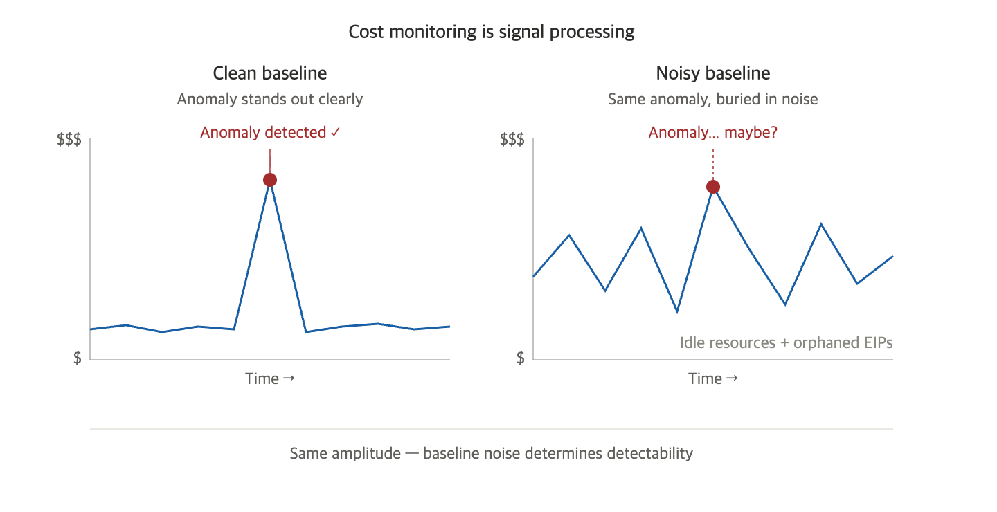
Consider an electrocardiogram. A normal heartbeat flows with small amplitudes on a steady baseline. If an arrhythmia occurs, a sharp spike clearly stands out. Doctors perform emergency treatment based on this spike.

But what if the machine itself is generating noise, causing the baseline to fluctuate? Even if the same arrhythmia occurs, it might be obscured by the noise and become invisible. The patient is put at risk, and the doctor detects the anomaly late.

Cloud costs have exactly the same structure:

Baseline — Normal costs incurred during regular operations
Signal — True anomalies that need to be caught (traffic spikes, incorrect deployments, resource surges due to security incidents)
Noise — Undeleted resources, floating EIPs, forgotten GPUs, unowned assets

Anomaly detection is ultimately determined by the Signal-to-Noise Ratio (SNR). If the noise is high, the same signal gets buried. Therefore, the true value of cleaning up undeleted resources is not cost savings, but “maintaining a clean baseline to quickly detect anomalies.”

Thus, Key Metrics Have Shifted

Traditionally, a “department good at budget management” was one with high forecast accuracy. However, in the cloud era, a “well-managed cost organization” is measured by different metrics:

MTTD (Mean Time To Detect) — Time taken from cost anomaly occurrence to detection
Variance Explainability — To what extent can the difference from the forecast be explained?
Tagged Coverage Ratio — The percentage of total costs for which an owner is clearly identified
Idle Resource Ratio — The percentage of resources that are not being used

The ±5% accuracy is gone, replaced by metrics like “detection within 24 hours” and “over 90% tag coverage.”

4 Patterns for Maintaining a Clean Baseline in Practice

① Automate Daily Cost Review

Ensure that “yesterday’s cost + 7-day average + difference %” is automatically posted to Slack every morning. Manual daily console monitoring is never sustainable.

# AWS CLI — Simple example to get yesterday's cost
aws ce get-cost-and-usage 
  --time-period Start=$(date -d 'yesterday' +%Y-%m-%d),End=$(date +%Y-%m-%d) 
  --granularity DAILY 
  --metrics UnblendedCost

② Enable Cost Anomaly Detection

AWS Cost Anomaly Detection, Azure Cost Management Anomaly, GCP Recommender — these are free features that can be enabled with a few clicks. Initially, set thresholds conservatively (e.g., exceeding 30% of the daily average) and adjust them based on alert fatigue.

③ Weekly Variance Review

Every week for 30 minutes, the infrastructure team and finance personnel meet to review the previous week’s Variance. Classify the causes of differences into three categories:

Normal business fluctuations (traffic increase)
Intended changes (new feature release)
Abnormal (incidents, undeleted resources, incorrect deployments)

Only the third category becomes an action item.

④ Regular Noise Cleanup

Clean up idle resources weekly or bi-weekly. What’s important here is a shift in perception:

We clean not to reduce costs, but to see the signal.

This framework must be shared across the entire team for a cleanup culture to be sustainable.

⚠️ Common Pitfalls

Obsession with accurate forecasting — If accuracy is forced, someone will start lying.
Quarterly reviews — For the cloud, quarterly reviews are too late. Daily/weekly is the standard.
Setting alarm thresholds too conservatively — If alert fatigue builds up, even real alerts will be ignored.
Refining prediction models while neglecting noise — If SNR is low, no model will work.
Viewing Variance as simple error — Variance is a learning signal. It should be an input for the next cycle.

✅ Summary

Cloud costs are about signal processing, not budget management.
Accurate forecasting is an illusion; the real goal is “narrow acceptable range + rapid detection.”
The operating model is a short cycle of Forecast → Observe → Adjust.
Key metrics have shifted from Forecast Accuracy to MTTD, Tagged Coverage, and Idle Ratio.
The real crime of undeleted resources is not the cost itself, but that they become noise that obscures the signal.

Making mistakes is normal. Not knowing is an incident.