When an LLM generates a sentence, it appears to naturally select the next word while remembering what it has already read. However, a Decoder-only Transformer does not contain a memory device like a human’s ability to recall sentences.
Instead, each token is transformed into vectors called Query, Key, Value, or Q·K·V for short. The Q at the current position calculates relevance with the K’s of previous tokens, and by bringing in more V’s from highly relevant tokens, it constructs the context.
This is combined with KV Cache to speed up inference. It’s a method of storing the K and V of already processed tokens and reusing them when generating the next token.
In this article, we will examine the entire process, from how Q·K·V are created, to Self-Attention calculation, Prefill and Causal Mask, token-by-token decoding, and the impact of KV Cache on performance.
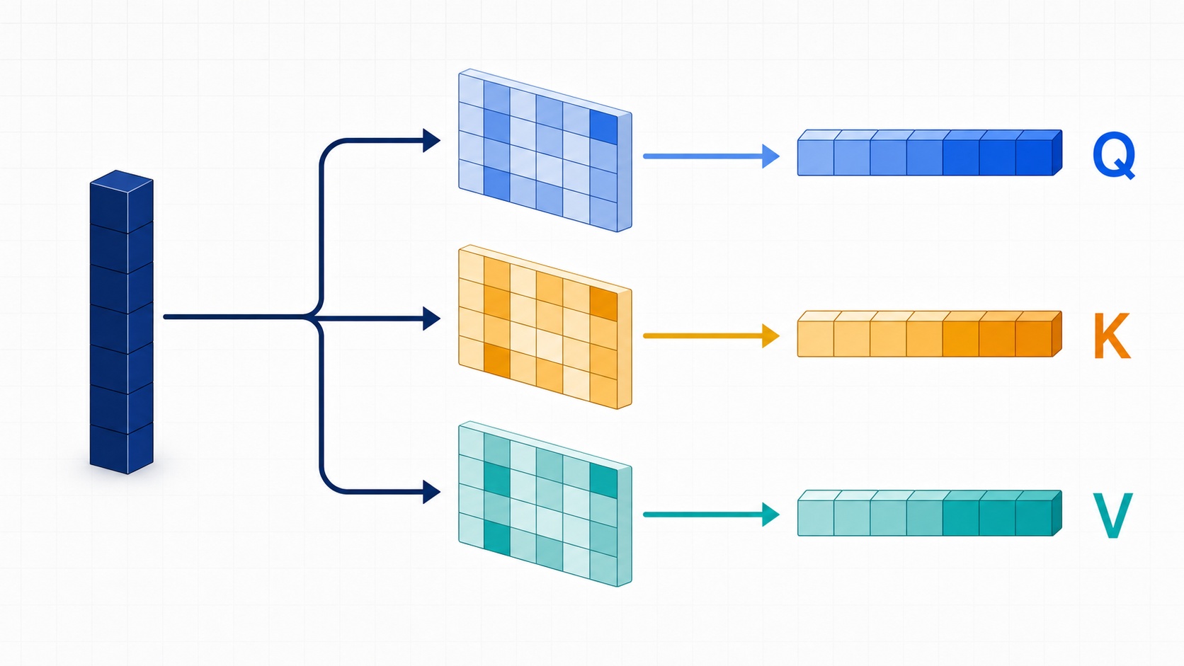
Figure: The three-pronged projection process where Q·K·V are created from a single token representation
Where Do Q·K·V Emerge From?
A Decoder-only Transformer is a stacked structure of multiple Transformer Layers. Each layer contains Self-Attention and a Feed Forward Network.
Q·K·V appear within Self-Attention. The important point is that Q·K·V are not created just once for the entire input sentence, but rather, each layer re-projects its current input to create new Q·K·V.
If the token representation entering a layer is X, it can be expressed as follows:
Q = XWQ
K = XWK
V = XWV
WQ, WK, WV are different weight matrices determined through training. Even when using the same token representation X, different vectors are created depending on the perspective from which comparisons are made and what information is to be conveyed.
토큰의 현재 표현 X
 ├─ WQ와 곱함 → Q
 ├─ WK와 곱함 → K
 └─ WV와 곱함 → V
It’s easy to understand these three vectors by likening them to a search system.
| Vector | Role in Attention | Search System Analogy |
| — | — | — |
| Q, Query | Information the current position wants to find | Search query |
| K, Key | Indicator of what information each position is related to | Document index/keywords |
| V, Value | Information actually delivered when selected | Document body |
However, this analogy should not be taken too literally. K does not store human-readable keywords, nor does V store sentences verbatim. Both are learned high-dimensional vectors, internal representations optimized for the model to perform its tasks.
Q Compares K and Retrieves V
The core of Self-Attention can be summarized in one sentence:
Using the Q at the current position, compare it with the K’s of all allowed positions, and then weighted-sum the V’s according to those scores.
Q and K are a pair for calculating relevance, and V is the information actually blended after relevance is calculated. Distinguishing these roles naturally helps understand why K and V are cached, while Q is typically not.
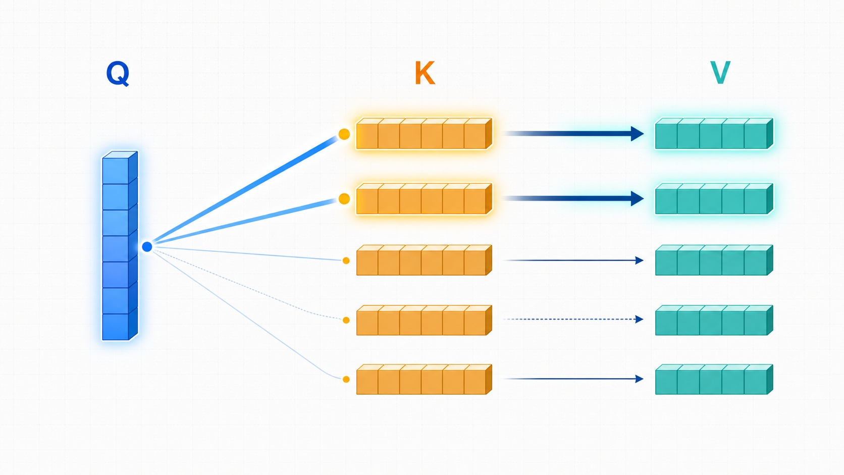
Figure: The process by which the reflection weight of V is determined as the comparison strength between Q and K changes
For example, let’s say we are processing the following sentence:
대한민국의 수도는 서울이다If we calculate the representation for the “Seoul” position during prefill or training, Q_Seoul can compare itself with the K’s of preceding tokens.
Q서울 · K대한민국 → 국가 문맥과의 관련도
Q서울 · K수도     → 수도 개념과의 관련도
Q서울 · K는       → 문법적 관계와의 관련도
Q서울 · K서울     → 현재 위치 자체와의 관련도
Let’s assume the relevance scores have been normalized as follows:
대한민국의 K → 0.30
수도의 K     → 0.50
는의 K       → 0.10
서울의 K     → 0.10
Then, the Attention output for the “Seoul” position can be thought of as the following weighted sum:
Attention 출력
= V대한민국 × 0.30
 + V수도    × 0.50
 + V는      × 0.10
 + V서울    × 0.10
This result is passed to subsequent calculations such as Residual Connection, normalization, and Feed Forward Network. As it passes through multiple layers, the token representation increasingly reflects the surrounding context.
Here, one distinction must be made. If the model has not yet generated “Seoul,” then the Q for the future token “Seoul” does not exist. In that case, the probability of the next token “Seoul” is predicted using the representation of the last token position in the prompt. The explanation of Q_Seoul applies to situations where the “Seoul” token is already included in the input or when its contextual representation is calculated after it has been generated.
How is Scaled Dot-Product Attention Calculated?
The representative formula for Attention is as follows:
Attention(Q, K, V)
= softmax(QKᵀ / √dₖ + M) V
Here, dₖ is the dimension of the Key vector used in one Attention Head, and M is the Attention Mask. The Causal Mask in Decoder-only models adds a very large negative number, conceptually -∞, to the scores of future positions, making the Softmax result 0.
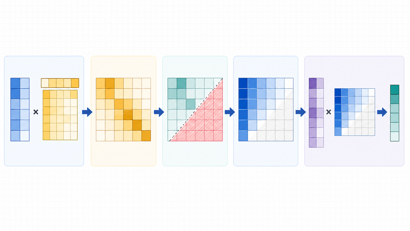
Figure: Attention pipeline leading from score matrix generation, scaling, Causal Mask, Softmax, to V weighted sum
The calculation can be divided into the following steps:
1. Create relevance scores by taking the dot product of Q and K
scores = QKᵀThe dot product of one row of Q and one row of K becomes the relevance score between the two vectors. When multiple tokens are calculated at once, a matrix containing scores between tokens is created.
2. Divide by √dₖ
As the vector dimension increases, the magnitude of the dot product can also increase. If scores become excessively large, Softmax can become saturated towards one side, leading to unstable training. Therefore, the magnitude is scaled by dividing by √dₖ.
scaled_scores = scores / √dₖ3. Apply the Mask
Decoder-only models must predict the next token, so they should not refer to future tokens that are after the current position.
allowed position → 점수 유지
future position  → -∞를 더함
4. Create weights with Softmax
weights = softmax(masked_scores)The scores in each row are converted into weights that sum to 1. Weights for future positions become 0, and weights for highly relevant past and current positions increase.
5. Weighted-sum V
context = weights × VThe final result is a new contextual vector that reflects more of the highly relevant Values.
What Changes in Multi-Head Attention?
Actual Transformers do not compare Q·K·V from just one perspective. Multiple Attention Heads learn relationships in different subspaces.
Some Heads might strongly focus on grammatical dependencies, while others might better capture relationships between distant subjects and predicates or the repetition of specific entities.
Head 1 → Q1, K1, V1 → Attention 결과 1
Head 2 → Q2, K2, V2 → Attention 결과 2
Head 3 → Q3, K3, V3 → Attention 결과 3
...
Concatenating the results of each Head and passing them through the output projection matrix WO yields the Multi-Head Attention output for the layer.
MultiHead(Q, K, V)
= Concat(head1, head2, ..., headh) WO
In modern LLMs, not only MHA (Multi-Head Attention) where every Query Head has independent K·V Heads is used, but also GQA (Grouped Query Attention) or MQA (Multi-Query Attention) where multiple Query Heads share K·V. This structure plays a crucial role in reducing KV Cache size and memory bandwidth.
Prefill Stage: Process the Entire Prompt at Once
Let’s assume the input is as follows:
생성형 AI는 문장을The tokenization result can be simply expressed as:
생성형 / AI / 는 / 문장 / 을In the Prefill stage, the GPU processes all tokens of the prompt in parallel. Each layer creates Q·K·V for all positions and calculates Self-Attention with the Causal Mask applied.
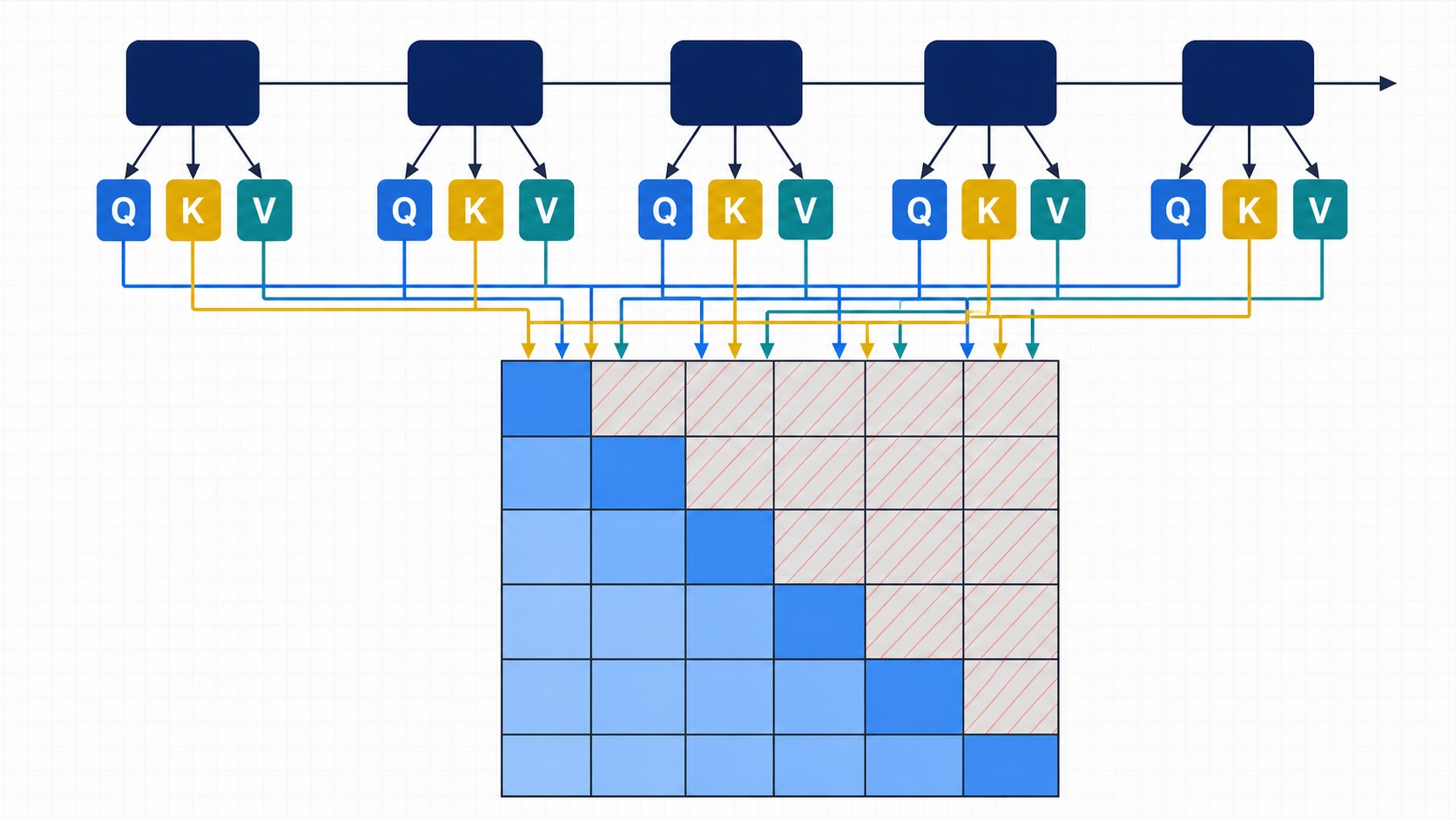
Figure: Prefill, where Q·K·V for all prompt positions are calculated in parallel, but future positions are blocked by a triangular Mask
생성형 → Q1, K1, V1
AI     → Q2, K2, V2
는     → Q3, K3, V3
문장   → Q4, K4, V4
을     → Q5, K5, V5
The range that can be referred to at each position is as follows:
Q1 → K1
Q2 → K1, K2
Q3 → K1, K2, K3
Q4 → K1, K2, K3, K4
Q5 → K1, K2, K3, K4, K5
In matrix terms, only the lower triangle is allowed.
        K1  K2  K3  K4  K5
Q1      O   X   X   X   X
Q2      O   O   X   X   X
Q3      O   O   O   X   X
Q4      O   O   O   O   X
Q5      O   O   O   O   O
Once Prefill is complete, the K and V of the prompt tokens from each layer are stored in the KV Cache. When calculating the probability of the next token, the Logits from the final Hidden State of the last input position are typically used.
생성형 AI는 문장을
→ 다음 토큰 후보의 확률
→ "처리" 선택
Prefill is a phase that actively utilizes GPU computation by allowing many tokens to be calculated in parallel. It is closely related to TTFT, Time To First Token, which is why the first token appears late when reading long prompts.
Decode Stage: Generate New Tokens One by One
Let’s say “처리” (processing) was selected as the first output token. In the next Decode Step, instead of feeding the entire prompt back into the model, only the new token “처리” is input.
Each layer calculates the Q·K·V for the new token.
"처리"
→ q6, k6, v6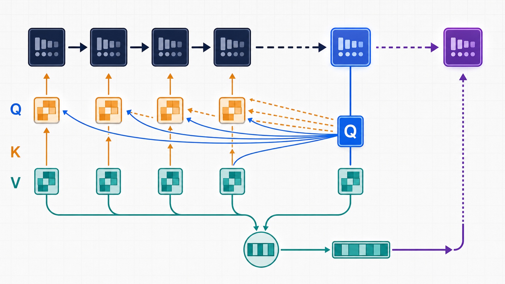
Figure: Serial Decode process where the Q of a single current token queries past K’s and weighted-sums V’s to generate the next token
In the current layer, q6 compares itself with both the past K’s stored in the cache and the new k6.
q6
→ [k1, k2, k3, k4, k5, k6]과 비교
With those scores, it weighted-sums the past and current V’s.
[v1, v2, v3, v4, v5, v6]
→ Attention 가중합
→ "처리" 위치의 문맥 벡터
After this calculation passes through all Transformer Layers, the final Hidden State is transformed into Logits of vocabulary size.
문맥 벡터
→ LM Head
→ 다음 토큰별 Logit
→ Softmax 또는 Sampling
→ "한다" 선택
Now, the same process is repeated with “한다” (do) as input. This method of using previously generated tokens as input again to generate the next token one by one is called Autoregressive Decoding.
Unlike Prefill, Decode requires the next step to wait for the result of the previous step. Tokens cannot be generated completely in parallel, and the KV Cache must be read at each step, so it is heavily affected by memory bandwidth and per-token latency.
What Does KV Cache Store?
KV Cache is a memory that stores the Key and Value of already processed tokens on a per-layer basis.
Layer 1 KV Cache
K1, K2, K3, K4, K5
V1, V2, V3, V4, V5

Layer 2 KV Cache
K1, K2, K3, K4, K5
V1, V2, V3, V4, V5

...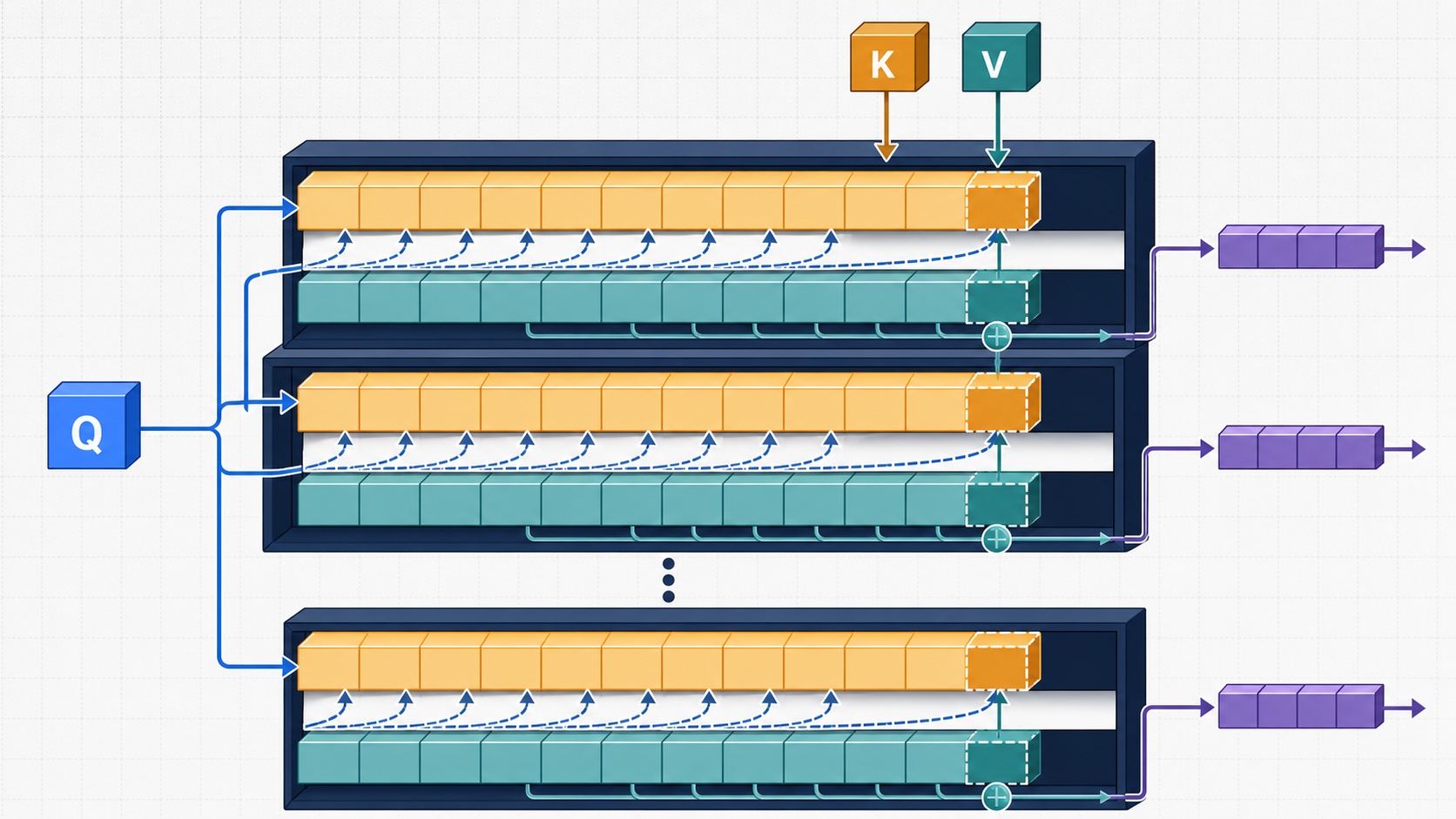
Figure: KV Cache, which re-reads past K·V stored per layer and appends only the new K·V of the current token to the end
When a new token arrives, each layer adds only the K and V of that token to the cache.
Kcache ← concat(Kpast, k현재)
Vcache ← concat(Vpast, v현재)
The Q of the current token is used immediately for Attention calculation but does not need to be reused in the next token step.
| Vector | Current Decode Step | Processing in Subsequent Steps |
| — | — | — |
| Current Q | Calculates relevance with cached K | Generally not stored |
| Current K | Compares with current Q | Added to KV Cache |
| Current V | Participates in weighted sum of current output | Added to KV Cache |
| Past K·V | Queried by current Q | Repeatedly reused from cache |
| Past Q | Not used | No need to recalculate or store |
The overall flow is as follows:
현재 토큰
  ↓
q현재, k현재, v현재 계산
  ↓
q현재 × [K과거 + k현재]ᵀ
  ↓
Attention 가중치
  ↓
[V과거 + v현재] 가중합
  ↓
현재 위치의 문맥 벡터
  ↓
다음 토큰 확률 계산
What Calculations Would Be Repeated Without KV Cache?
Without KV Cache, every time a token is generated, the entire sequence processed so far would have to be re-processed.
첫 번째 생성
프롬프트 전체 계산

두 번째 생성
프롬프트 + 첫 출력 전체 계산

세 번째 생성
프롬프트 + 첫 출력 + 두 번째 출력 전체 계산
Using KV Cache allows for the reuse of K and V projection results from already processed positions.
첫 번째 생성
프롬프트의 K·V 저장

두 번째 생성
새 토큰의 q·k·v만 계산
+ 과거 K·V 재사용

세 번째 생성
다시 새 토큰의 q·k·v만 계산
+ 더 길어진 과거 K·V 재사용
However, KV Cache does not make Attention calculation entirely constant-cost. A new Query still needs to compare with more past Keys and read more Values as the sequence lengthens.
없어지는 비용
→ 과거 토큰의 K·V를 다시 투영하는 계산

남아 있는 비용
→ 현재 Q와 전체 캐시 K의 비교
→ 전체 캐시 V의 가중합
→ 길어진 Cache를 읽는 메모리 비용
In other words, while KV Cache significantly reduces redundant calculations, it does not eliminate the problem of increased Attention lookup volume and memory usage as the context lengthens.
Why Does KV Cache Memory Grow?
The basic KV Cache size is proportional to the following factors:
KV Cache 크기
≈ 2
× Transformer Layer 수
× KV Head 수
× Head 차원
× 저장 토큰 수
× 배치 크기
× 원소당 바이트
The ‘2’ in front is because both K and V are stored. If the context lengthens or the number of concurrent requests increases, the Cache can grow rapidly.
Therefore, the following optimizations are used in actual LLM Serving:
- Reduce KV Head count with GQA·MQA
- Quantize KV Cache to lower precision
- Offload some layer Caches to CPU
- Limit older token range with Sliding Window Attention
- Manage Cache memory in pages with Paged Attention
- Reuse KV Cache of common Prefixes across multiple requests
Each method involves trade-offs between speed, memory, accuracy, and implementation complexity.
Common Misconceptions When Understanding KV Cache
KV Cache is not the model’s long-term memory
KV Cache is an intermediate result for Attention of tokens already processed in the current request. When the conversation ends and the Cache is discarded, no new knowledge remains in the model parameters.
Cache does not store only raw token text
It’s not a simple record of token IDs or strings, but rather the K·V Tensors calculated in each Transformer Layer are stored. Therefore, model size, layer structure, and the number of KV Heads directly affect memory usage.
If a past sentence changes, the Cache cannot be used as is
KV depends on previous tokens, positional information, and calculations from preceding layers. If tokens in the earlier part change, the subsequent Cache no longer represents the same context, so everything after the point of change must be re-calculated.
KV Cache is primarily for inference
During training, the gradients for the entire sequence must be calculated, so a typical generative KV Cache is not used in the same way. Hugging Face documentation also advises that Cache should be used for inference.
Summarizing Again in One Scene
Connecting Q·K·V and KV Cache in chronological order is as follows:
1. 프롬프트 토큰화
2. Prefill에서 모든 프롬프트 위치의 Q·K·V 계산
3. Causal Mask를 적용해 미래 토큰 참조 차단
4. 각 레이어의 프롬프트 K·V를 Cache에 저장
5. 마지막 위치의 Logits로 첫 출력 토큰 선택
6. 새 토큰의 q·k·v만 계산
7. q로 캐시된 K를 조회하고 V를 가중합
8. 새 k·v를 Cache 끝에 추가
9. 다음 토큰을 선택하고 6번부터 반복
The core points, compressed, are as follows:
Q is the vector that asks what the current position should refer to, K indicates what information each position is related to, and V is the information actually delivered when selected.
And the core from an inference performance perspective is as follows:
The K and V of past tokens are stored in the layer-specific KV Cache for reuse, and only the K and V of the current token are added whenever a new token is generated. However, the new Q still needs to query the K and V of the entire Cache, so the computational load and memory cost for long contexts are not entirely eliminated.
Q·K·V can be understood as the principle by which LLMs select context, and KV Cache as an inference optimization that allows this selection to be repeated at a realistic speed for each token.
Leave a Reply