🔍 Mastering OpenTelemetry: A Complete Guide to Metric Views

Hello! Today, we’re going to dive deep into one of OpenTelemetry’s powerful features: Metric Views. Have you ever wished you could customize your collected metric data before sending it to the backend? That’s exactly what ‘Metric Views’ are for – your secret weapon! 🚀

###

What are OpenTelemetry Metric Views?

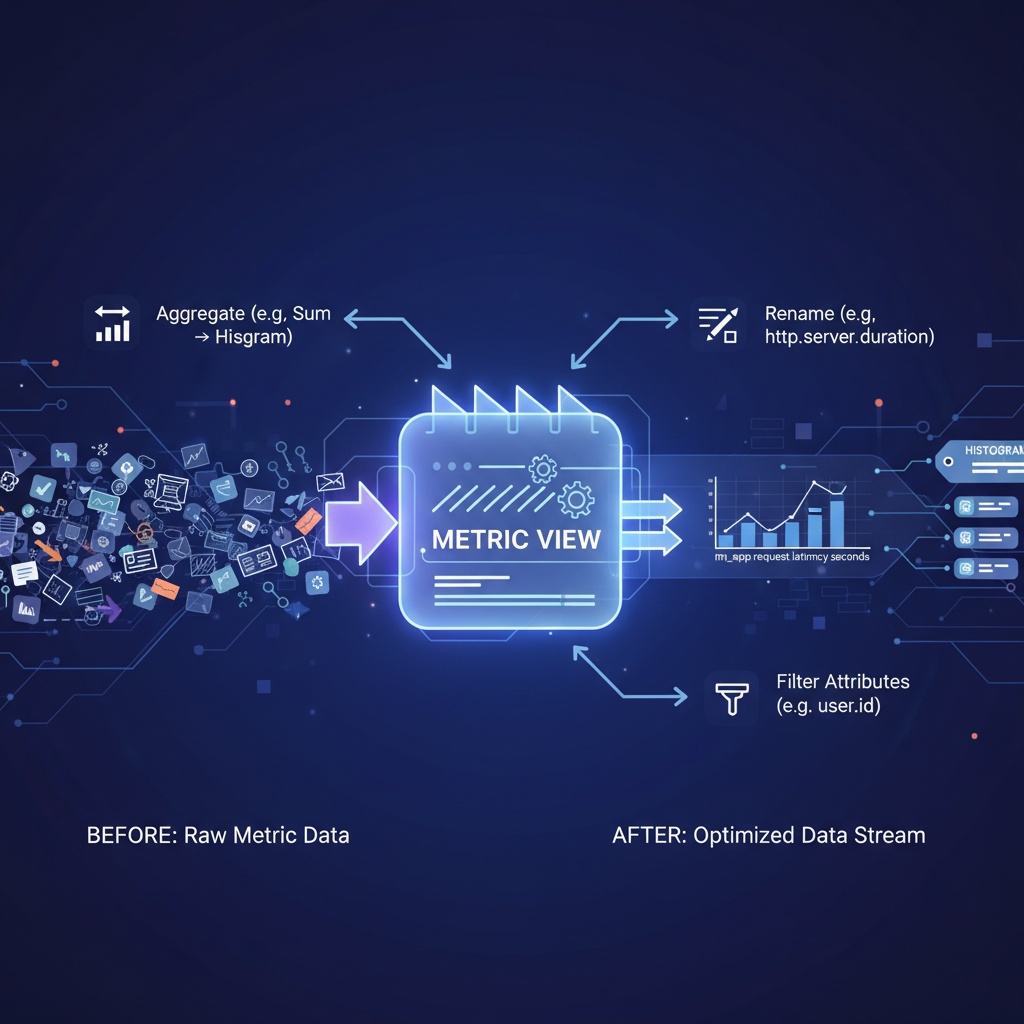
Simply put, Metric Views can be described as a ‘data customization workshop’ operating at the heart of the OpenTelemetry SDK. 🏭

Just before the metric data we diligently collect from our applications departs for its final destination (e.g., Prometheus, Datadog), it passes through a gateway called ‘Metric Views’. At this gateway, we gain the powerful ability to freely change the data’s shape, filter it, or reconfigure it.

In other words, it’s a core mechanism for customizing and transforming metric streams before the data is sent externally via an Exporter.

Metric Views are a powerful feature that allows you to process and control metric data before it’s sent to the backend. You can select specific metrics and perform the following operations:

• Change Aggregation: You can change the default aggregation method (e.g., sum, last value) to a histogram or another method. For example, you can collect HTTP request durations as a histogram instead of the default aggregation to understand their distribution.
• Filter Attributes: You can add or exclude specific attribute keys to save storage space and retain only the data necessary for analysis. For example, you can exclude high-cardinality attributes like http.client_ip to reduce costs.
• Rename and Add Description: You can rename metrics to be clearer or add descriptions to improve readability.
• Select Instruments: You can apply views only to instruments with specific names, types, or units.

✨ Amazing Things You Can Do with Metric Views

With Metric Views, you can perform a variety of tasks. Shall we look at them one by one?

1. Change Aggregation Method for Specific Metrics 📊 ➡️ 📈

This is one of the most powerful features! For example, let’s say you have a request count metric that is aggregated as a ‘Sum’ by default. However, you might want to know not just the total sum, but how requests are distributed across different time periods. With Metric Views, you can easily change the aggregation method for this metric to a ‘Histogram’.

• Before: request_count (simple sum)
• After (with View): request_count (histogram showing distribution over time)

2. Rename Metrics 🏷️

There are times when you need to adhere to an organization’s metric naming conventions or change metric names for compatibility with existing systems. Metric Views allow you to cleanly rename the original metric names generated at the code level to your desired names before exporting them.

• Before: http.server.duration
• After (with View): my_app.request_latency_seconds

3. Filter Unnecessary Attributes 🧹

Metric data is collected along with various context information in ‘Attributes’ (e.g., http.method, http.status_code, user.id, etc.). However, sometimes too many attributes can lead to an explosive increase in data cardinality, causing cost issues or performance degradation. Metric Views act as a savior in such cases! You can selectively remove attributes deemed unnecessary, leaving only the essential data.

• Before: metric{user_id=”123″, client_ip=”…”, …}
• After (with View): metric{…} (sensitive or unnecessary attributes removed)

4. Set Histogram Bucket Boundaries 📏

Histograms are powerful tools for showing data distribution, but how you divide the intervals (buckets) is crucial. If our service’s response time (latency) is mostly under 100ms, but the histogram buckets are set too wide, like [1s, 2s, 5s, …], meaningful analysis would be difficult. With Metric Views, you can finely adjust histogram bucket boundaries to values optimized for your service.

• Default Buckets: [0, 5, 10, 25, 50, …]
• Custom Buckets (with View): [0.01, 0.05, 0.1, 0.25, 0.5, 1] (more granular analysis possible)

---

💡 Why are Metric Views Important?

In conclusion, Metric Views empower us to perfectly control the Shape, Granularity, and Cardinality of our data before it’s sent to our observability backend.

This provides us with the following benefits:

• Cost Savings 💰: Reduce transmission volume and storage costs by filtering unnecessary data.
• Performance Improvement ⚡️: Reduce the load on backend systems, enabling faster and more efficient data processing.
• Increased Analysis Efficiency 🎯: Process data to suit analysis objectives, yielding more meaningful and accurate insights.

---

How to Configure Metric Views

Metric Views are typically configured when setting up the MeterProvider. Most language SDKs offer similar concepts, and here we’ll explain the conceptual flow along with code examples.

1. Registering Views

Register one or more views with the MeterProvider to control metric streams.

Conceptual Procedure:

1. Instrument Selector: Select which instrument(s) to apply the view to. You can specify by name, type, meter name, etc.
2. Stream Configuration: Define how to process the selected instrument data stream. This includes setting a new name, adding a description, filtering attributes, and changing the aggregation method.
3. Add View to MeterProvider: Register the created view with the MeterProvider.

2. Key Components

Instrument Selector

Rules for selecting the target to which the view will be applied. You can select based on various criteria.

• instrument_name: Name of the instrument (e.g., http.server.duration)
• instrument_type: Type of the instrument (e.g., Histogram, Counter, Gauge)
• meter_name: Name of the Meter that created this instrument
• meter_version: Version of the Meter

You can also use wildcards (*) to apply rules to multiple instruments (e.g., http.*.duration).

Stream Configuration

Defines how to process the selected metric data.

• name: New metric name
• description: Description for the metric
• aggregation: Defines the aggregation method (see ‘Aggregation Methods’ below)
• attribute_keys: List of attribute keys to collect. Keys not in this list will be removed.

3. Aggregation Methods

The main aggregation methods available in views are as follows:

• SumAggregation: Calculates the sum of all measurements. (Default for Counter)
• LastValueAggregation: Uses the last measured value. (Default for Gauge)
• DropAggregation: Completely removes the metric.
• ExplicitBucketHistogramAggregation: Creates a histogram based on user-defined boundary values. This allows for visualizing the distribution of values.
• Example: [0, 5, 10, 25, 50, 100] to understand response time distribution in milliseconds (ms)

---

Code Example (Python)

The following is an example of aggregating the http.server.duration metric as a histogram and removing unnecessary attributes in the Python OpenTelemetry SDK.

from opentelemetry import metrics
from opentelemetry.sdk.metrics import MeterProvider
from opentelemetry.sdk.metrics.view import View, InstrumentSelector
from opentelemetry.sdk.metrics.aggregation import ExplicitBucketHistogramAggregation
from opentelemetry.sdk.resources import Resource

# 1. Create View
# Select http.server.duration metric and change aggregation method to histogram
histogram_view = View(
    # Select instrument named 'http.server.duration'
    selector=InstrumentSelector(
        instrument_name="http.server.duration",
        instrument_type=metrics.Histogram
    ),
    # Set new name and description
    name="http.server.duration.histogram",
    description="Duration of inbound HTTP requests in milliseconds",
    # Change aggregation method to explicit bucket histogram
    # Aggregate response times into 0, 10, 50, 100, 500ms boundaries
    aggregation=ExplicitBucketHistogramAggregation(
        boundaries=(0, 10, 50, 100, 500)
    )
)

# 2. Register View with MeterProvider
resource = Resource.create({"service.name": "my-service"})
meter_provider = MeterProvider(
    resource=resource,
    views=[histogram_view] # Register the created view
)

# 3. Set MeterProvider globally
metrics.set_meter_provider(meter_provider)

# When metrics are recorded in the application code later
# The http.server.duration metric will be processed according to the view rules defined above.
meter = metrics.get_meter("my-app.meter")
histogram = meter.create_histogram(
    "http.server.duration",
    unit="ms",
    description="HTTP server request duration"
)

# ... Application logic ...
# histogram.record(request_duration_in_ms)

By leveraging Metric Views in this way, you can flexibly control the format and content of collected metric data without changing application code, which is very useful for optimizing the efficiency and cost of your monitoring system.

If you are using OpenTelemetry, actively utilize Metric Views to upgrade your observability data to the next level!

---